Author Archives: t.fujisawa

Problems on the plot and summary functions

I have recently received reports from multiple users that the plot and summary functions for the GMCY stopped working in the R version 4.0 or later.

This is due to the changes on the function naming rules introduced in R 4.0.

The problem is fixed in the splits version 1.0-20. If you use R 4.0 ( or later), please update the splits package to 1.0-20.

https://r-forge.r-project.org/R/?group_id=333

How tr2-delimitation over-splits structured populations – a case of unresolved trees

I recently wrote a blog post about the effect of reduced gene flow over the multilocus species delimitation program, tr2. A general pattern is, even if two populations are connected with moderate gene flow, the tr2 erroneously splits them into two “species” when a very large number of loci are used. This result means we need to be cautious when we apply it to a big data set.

One thing I didn’t test is that the effect of unresolved gene trees. In the previous post, I assumed  gene trees are fully resolved. This assumption is rarely met in real data sets as RAD markers or exons of RNAs are not variable enough to give us fully resolved trees. Does this also affect the patterns of oversplits of tr2?

I just tested the effects of less-variable markers on tr2-delimitation. The simulation setting is identical to the previous post except that the branch lengths of gene trees are proportional to mutation rate. As mutation rate gets smaller, gene trees are more unresolved.

The gene trees simulated under Neμ= 0.005 are plotted below. They look realistic, just like gene trees we see in real practices. (You may think that these trees are not informative enough to detect recent speciation. Actually, they are informative.)

genetrees.nemu0.05

So, how does tr2 oversplit populations connected by gene flow, and how does mutation rate affect the pattern of oversplits?

species_tree.svg

The above plot is a species-population tree used in simulations. Pop.1 and pop.2 are connected by gene flow.

The plot below shows the proportions of trials where samples from two populations were assigned to one species. The migration parameter is Nem=1.0, and population mutation parameter, Neμ, ranged from 0.005 to 5.

p.n.vmu

The pattern of oversplits is similar to the previous simulations (see the plot). When Neμ= 0.5 or 5, curves are almost identical to the curve with fully-resolved gene trees. With > 500 loci, populations are always split into two “species”. When you have less mutations, curves diverged from the ideal curve and the overspliting slows down.

This is probably a good result. At least, less informative markers don’t lead you to false positives. However, they are probably less sensitive to the true pattern and you may miss it.

When you use tr2-delimitation, maybe you need to consider two points: how informative your markers are and how many markers you use. As you increase the number and informativeness of loci, you can detect finer scale structure, which may or may not be true species.

Again, it is often hard to determine the “sweet spot” of numbers and variability of markers to detect “true” species since speciation is always continuous. I am not sure if this problem can be solved by the delimitation with full multispecies coalescent model. (tr2 is an approximate method.) Explicit modeling of gene flow or geographic distribution is probably the better approach to tackle this problem, but usually time-consuming.  It may be possible to use resampling of loci to check how the pattern of splits develops, and combine it with locus informativeness to find the best threshold for true species entities.


A new transcriptome paper is published

A paper on transcriptome phylogeography of periodical cicada is now out.

Fujisawa, T., Koyama, T., Kakishima, S., Cooley, J. R., Simon, C., Yoshimura, J., & Sota, T. (2018). Triplicate parallel life cycle divergence despite gene flow in periodical cicadas. Communications Biology, 1(1), 26.

It is a detailed phylogeographic study of three species groups of Magicicada periodical cicadas. We found gene flows between geographically adjacent, closely related 13 year and 17 year species. We also searched for genes responsible for the life cycle control, but did not find any divergent loci shared by three species groups.

How tr2-delimitation over-splits structured populations

As I test the tr2-delimitation with more data sets and read more papers applying it to  difficult species, I find that it sometimes infers an unrealistically large number of species. These oversplits appear to happen more frequently when tr2 is used with very large data sets (like thousands of loci of RAD or RNA).

A reasonable explanation for this tendency of oversplit is tr2 delimits structured populations as species even if they are connected with gene flow. Whether molecular species delimitation methods actually delimits species or not is still under debate (like this paper). But, it is quite possible that tr2 falsely finds populations connected with weak gene flow as “species”.

The basic idea of tr2 delimitation is that sets of gene tree topology are more similar to each other when multiple species exist in your samples. This concordance of topology results in a skewed distribution of triplets, where one triplet topology is more frequently observed than other two.

Reduced gene flow between populations also creates topological concordance. The effect of reduced gene flow is usually much smaller than the effect of true speciation and often undetectable with a small number of loci. However, even a minimal skew of triplet distribution is detected as a signature of species when the number of  loci is VERY large.

Because the tr2’s triplet distribution model only considers triplets’ topology and  does not include the distribution of branch length, the gene flow likely has more significant effect on its performance than the full multi-species coalescent model (such as BPP).

I checked with simulations how reduced gene flow between populations affects the delimitation results of tr2.

Gene trees were simulated under a model where two populations split but retain genetic exchange with gene flow. The age of split, T, is nearly the same value of effective population size, Ne. For example, if Ne = 50,000 and generation time is 1 year, the time of split is 50,000 years ago. The amount of gene flow, Ne*m = 0.5, 1.0 and 5.0. In this simulation, gene tree’s topology is known without error. (I will consider situations with unresolved gene trees in future posts.)

species_tree.svg

Does tr2 split these two populations, pop.1 and pop.2,  into separate species?

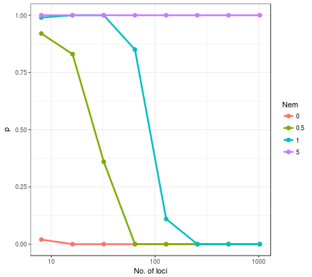
The plot below shows proportions of trials where samples from pop.1 and pop.2  are assigned to the same species and how the proportions change with the number of used loci. Different colors represent different degrees of gene flow.

p.n

As you can see, even under conditions with moderate gene flow (Nem=0.5 or 1), samples from two populations were split into two spurious species. For example, populations connected with gene flow of Nem=1.0 were always split into two species when the number of loci exceeded ~500.

With Nem=5, which means gene flow is very large, the tr2 did not split populations even with 1000 loci (, but I guess it will probably oversplit if much larger number of inputs are used). When Nem=0, that is, the two populations are truely two young species, just about 10 loci was enough to detect them.

The reduced gene flow does have a strong effect on delimitation. So, you need to be careful when interpreting the results of multilocus delimitation with a very large data set. Splits detected only with hundreds or thousands of loci  are probably not species, but population structure.

In the simulation above, only 10 or 20 loci with well-resolved tree topology have enough power to detect young species. Therefore, using different size of inputs and checking how patterns of split appear by increasing loci may help us interpret results.

Ultimately, it is quite hard to decide one threshold of gene flow and an appropriate sample size with which we can confidently say “there are species” since speciation process is continuous. Also, variation of informativeness of loci makes this decision even more difficult (You need more loci when they are less informative).

It seems that explicit modelling and quantification of gene flow is a better way to tackle this problem and should be a new direction of the multilocus delimitation program.

Superimposing maps of two cities with ggmap

I recently moved from Kyoto to Paris to do my second postdoc. In the process of flat hunting in Paris, which has been very hard  because of  the rising housing cost, I walked around some different parts of Paris. One impression I had is Paris is small. Once you walk through the city,  you will find this quite easily.

My intuition told me that its size is almost close to the size of Kyoto, which is a medium-sized city in Japan. But, is it true? I found a website comparing London and Paris, and it says London is larger than Paris, but no comparison between Paris and Japanese cities exists.

So, I just checked by superimposing maps of the two cities. I used an R package called “ggmap”, a very nice geographic visualization package built based on ggplot2.

I first downloaded maps of Paris and Kyoto in 15km squares surrounding city centers. (I chose the Cite island for Paris and Shijo-Karasuma for Kyoto as centers). This process was a bit tricky because maps are defined by longitudinal and latitudinal range. The identical longitudinal ranges do not represent the same distance when the cities’ latitudes are different. I used the “great circule distance” equation to adjust the effect of latitude on the longitudinal distance and and find appropriate ranges.

R <- 6371
#convert distance to longitudinal range given a latitude
delta.lambda <- function(d, phi=0.0) {
	2*asin(sin(d/R/2)/cos(phi))
}

#create longitudinal and latitudinal ranges which define a suquare with length d
map.range <- function(d, lat=0.0, lon=0.0){
	dphi <- d/R*360/2/pi
	dlambd <- delta.lambda(d, phi=lat*2*pi/360)*360/2/pi

	lonrange <- lon + c(-dlambd/2, dlambd/2)
	latrange <- lat + c(-dphi/2, dphi/2)

	rang <- c(lonrange, latrange)
	names(rang) <- c("left", "right", "bottom", "top")
	return (rang)
}

In the above code, the map.range function returns longitudinal and latitudinal range which covers a square with its side length = d km.

Once you can define a range to draw, downloading and plotting maps is simple thanks to ggmap functions.

d <-15 #15kmx15km map
z <- 12 #Zoom level
kyoto_center <- c(35.0, 135.76)
kyoto <- map.range(d, lat=kyoto_center[1], lon=kyoto_center[2])
kyoto_map <- get_stamenmap(kyoto, zoom=z, maptype="toner")
ggmap(kyoto_map)

paris_center <- c(48.855, 2.34)
paris <- map.range(d, lat=paris_center[1], lon=paris_center[2])
paris_map <- get_stamenmap(paris, zoom=z, maptype="toner")
ggmap(paris_map)

The “get_stamenmap” function downloads a map from Stamen Maps. If you like Google map, use “get_googlemap” function to download from Google map.
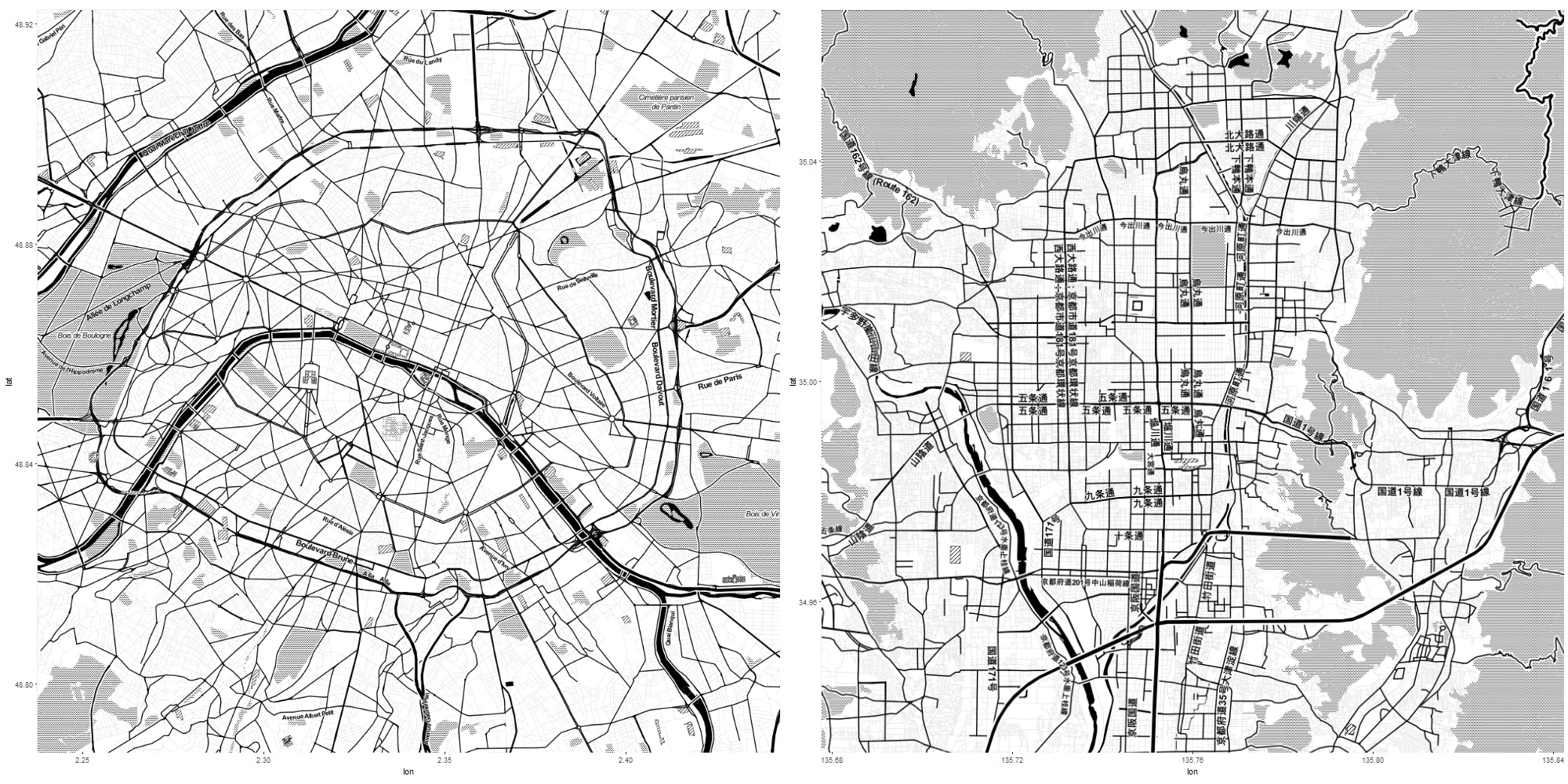
maps

The two maps plotted side by side tells me a lot. For examplem the Peripherique motor way, which defines Paris, looks quite similar size as the city of Kyoto surrounded by mountains.

Superimposing two maps was another tricky point. The ggmap has two ways for superimposition of graphics, “inset_map” and “inset_raster”. It seems “inset_raster” is an appropriate function because it allows me to set coordinates for regions you superimpose graphics. One problem is that it does not allow me to change alpha value. I just added alpha values to the raster graphics of the map and plot it using the inset_raster.

translucent.raster <- function(map){
	tmp <- as.matrix(map)
	tmp <- gsub("$", "55", tmp)
	tmp <- gsub("FFFFFF", "0000FF", tmp)
	ras <- as.raster(tmp)
	attributes(ras) <- attributes(map)
	ras
}

ggmap(paris_map) + inset_raster(translucent.raster(kyoto_map), xmin=paris["left"], ymin=paris["bottom"], xmax=paris["right"], ymax=paris["top"])

superimpose.02

This is a bit awkward way, but the result looks OK. Now, I can compare landmarks more precisely.

The Golden and Silver temples (indicated by small black arrows), which define north-west and north-east edges of Kyoto area are almost on the Peripherique. This means walking from the Cite island to the Peripherique is just like walking from Shijo-Karasuma to the Silver temple. Probably, this distance similarity made me feel that the two cities are in similar size.

Of course, Paris has much larger suburban area, and the size of Paris metropolitan area is much larger than Kyoto. But, my intuition looks more or less correct.