How to set up an environment for “tr2”

Installing Python and check versions

Python is required to run the tr2-delimitation on your computer. In many modern operating systems, Python is pre-installed and you do not need to install it by yourself.

However, the installed version of Python matters. The tr2 is written in Python 2,  while, in some recent systems, Python 3 is the default version. This is simply because Python 2 was a standard when I started writing the codes, but Python 3 is becoming a new standard now. (I am translating the tr2 codes into Python3.) So, you first need to check the version of Python installed on your system.

Type on your console,

$python --version

If you see a message like below, you are running Python 2.

Python 2.7.6

In some decent OS’s, both Python2 and 3 are pre-installed, and you can call Python 2 by

$python2

even when your default Python is Python3.

If your environment does not have Python2 at all, visit the Python website and install it, or create a Python2 environment as explained in the next section.

Installing dependencies (scipy/numpy and Java)

Python packages called numpy/scipy is required to run tr2. These packages are for numerical calculations. Visit SciPy website and follow the instructions for your operating system to install Scipy libraries. Installing all Scipy related packages following the instruction is just fine though not all Scipy packages are required to run tr2.

An alternative, easy way to install dependencies is installing an all-in-one suite like Anaconda, which includes Python and related packages. As Anaconda allows you to run multiple versions of Python, you can install it with any version of Python.

If you choose to install Anaconda with Python3, you must run Python2 codes by creating Python2 environment.

$conda create --name python2 python=2 numpy scipy

This “conda” command creates an “environment” where the python version is 2 with numpy/scipy installed. You can switch to it by calling the “activate”  command,

$activate python2

and switch back to the default environment by the “deactivate” command.

(python2) $deactivate

 

Checking packages

You can check if the packages are properly installed by loading them on the interactive shell.

$python

(Just by typing “python”, “interactive shell” starts. You can quit this mode by pressing Ctl+d.)

>>>import numpy, scipy

If it does not return errors, packages are ready to use.

Java is also required to run the consensus tree building program, triplec. Almost all modern operating systems have Java as pre-installed software.

Multilocus delimitation with very short sequences

Are very short sequences useful for species tree reconstruction and species delimitation?

Sequence fragments generated by some NGS platforms are often very short (for example, 100bp with RAD) and each locus contains only a few informative sites. Intuitively, they do not look useful for tree reconstruction using gene tree-based method (that is, species tree estimation using estimated gene trees. The SNP-based methods are not included in this category.) because tree of each locus is unresolved and uninformative for subsequent specie s tree inference.

I did a bit of simulation to check if the gene tree-based species tree reconstruction and delimitation work on very short sequences. Results are rather surprising.

The procedure of simulation is simple.

1. Set up a species tree.
2. Simulate 500 gene trees within the species tree assuming multispecies coalescent.
3. Simulate sequence alignments of 100bp along the gene trees.
4. Reconstruct gene trees.
5. Reconstruct a species tree.
6. Delimit species using the species tree as a guide.

The R codes are available here so you can replicate the simulation. You need following programs to replicate: fastsimcoal2, Seq-gen, RAxML, ASTRAL and tr2.

The species tree used for simulation is below. I set the effective population size for each species in between of T3 and T2. So, I expect large amount of incomplete lineage sorting among sp1, sp2 and sp3. Sample size from each species is 5.

The picture below shows simulated gene trees (upper row), simulated alignments (middle row) and reconstructed gene trees (bottom row) for three loci.

The sequences and reconstructed gene trees appear to be barely informative. Although some distantly related species are monophyletic even in reconstructed trees,  closely related ones are unresolved. The bottom left tree is almost “flat”.

The tree below is a species tree reconstructed by ASTRAL with 500 simulated loci, and a result of delimitation. The numbers on the nodes are scores of delimitation (positive values indicate nodes are between-species branchings, and “*” signs show species groups.)

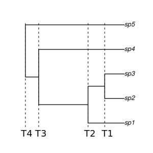
One surprising thing is that ASTRAL was able to reconstruct a correct species tree even with apparently uninformative gene trees. It seems delimitation with tr2 can work correctly too once the species tree is correctly estimated.

This is only one simulation run, but I am quite sure that even very short sequences contain information and can be useful with the gene tree-based reconstruction and delimitation, at least, under ideal conditions.

Of cause, real data contain lots of missing sites/loci. There may be gene flows. I guess the ideal conditions of multispecies coalescent are rarely met. I will test how the methods respond to the violations.

—

Update: 14/Sep/16

Some users of tr2 reported that it crashed when they input thousands of gene trees of RAD. I found that the numerical calculation underflows when the input is very large. I made some small fixes on the program, but it accepts only  about 1000 loci now.

I think the simulation above says even 500 loci can have enough information to delimit some difficult species. But, I am thinking of how to solve this limitation of the number of loci.

image.h.R: how to color your bases

I wrote a blog post about an R function to visualize an alignment matrix long time ago. I no longer use the function because the “ape” package now has a function, called “image.DNAbin”, which does exactly the same thing.

When I was analysing my SNP data, I found the image.DNAbin does not show ambiguous bases which represent heterozygous sites.

 

Although I can tell the function to show ambiguous letters, say, “Y” or “M”, in the image, it does not automatically assign colors to them.

If the ambiguous bases are colored by the “in-between” of two unambiguous bases, (say, if A is red and C is yellow, M=A/C is in an orangish color), the plot will be much more informative.

R has a function to generate colors between two colors, called “colorRamp”. It is an interesting function which returns a function to interpolate colors between two colors.

RY <- colorRamp(c('red', 'yellow'))
RY(seq(0, 1, 0.1))
      [,1]  [,2] [,3]
 [1,]  255   0.0    0
 [2,]  255  25.5    0
...
[10,]  255 229.5    0
[11,]  255 255.0    0

In the case above, the function “RY” returns RGB values interpolating red and yellow. You can convert these values into color codes by the “rgb” function. Using these functions, a nice color gradation is easily drawn.

g <- rgb(colorRamp(c('darkblue', 'lightblue'))(seq(0,1, 0.1)), max=255)
barplot(1:10, col=g, border=F)

 

Using the “colorRamp”, I wrote a simple code to generate 6 colors for heterozygous bases from 4 colors for unambiguous bases.

image.h <- function(sq, col=c('red','yellow','green','blue')) {
	bases <- c('a', 'g', 'c', 't')
	dbases <- c('r', 'm', 'w', 's', 'k', 'y')

	dcol <- apply(combn(col,2), 2, function(x){rgb(colorRamp(x)(0.6), max=255)})

	image(sq, col=c(col, dcol, 'lightgrey', 'black'), what=c(bases, dbases, 'n', '-'))
}

The four colors, red, yellow, green and blue, are colors for A, G, C, and T respectively. The “colorRamp” function in the fifth line generates 6 colors from the combinations of  the 4 colors.

The image drawn by the new function looks OK. The heterozygous sites are shown in reasonable colors, like orange, purple and bluish green.

However, there is one problem. The color for “K” is grey, which is the same color for “N”. This is because the colors for “G” and “T” are complementary and produce grey when they are mixed.

Is there a set of colors for AGCT which does not produce grey when they are mixed?

I guess the answer is no, at least with simple colors like red-green-blue and cyan-magenta-yellow.  Because when you choose 4 colors from these basic 6 colors, at least one pair is always complementary. (If you see an RGB cube, this is obvious. You can never choose 4 vertices  without including a pair of opposite ones. Black and white are not allowed.)

Interestingly, when I google color schemes for DNA bases, they often use complementary colors to show complementary bases, say, blue for A and yellow for T. I think this is an intuitive decision, but I want to avoid using the complementary colors for my function.

I found designing good color schemes for DNA bases is an interesting topic, and  it looks  very difficult to design schemes which are both informative and beautiful. A set of vivid, informative colors often contains complementary colors while restricting your color space to avoid using them makes the image opaque and less informative.

What I did in the script  is to use 0.6, instead of 0.5 for colorRamp argument not to take the exact mid points between two colors and to avoid producing the identical greys. But, probably, there must be better approaches.

 

Is your multilocus phylogeny correct?

I am now working on a transcriptome data set for a phylogenomic project. Building trees from huge multilocus data obtained by NGS is now widely practiced, but how reliably we can reconstruct phylogeny with them is still largely unknown.

In my data set, most loci are very little informative because sequences of exons are sometimes extremely conservative (the number of variable sites is often less than 1 in 1000bp). Some loci possibly span thousands of bases and the effect of recombination within locus may not be ignored. In addition, as is often the case with NGS data, they have a quite large number of missing sites and missing loci. I imagine that my transcriptome data boldly violate the common assumptions of phylogenetic inference.

Methods for tree inference also matter. Is concatenation of all loci better than using the multi-species coalescent methods? Do you Infer gene trees first or do all inference simultaneously?

To check the reliability of my phylogenetic inference, I searched recent papers reporting the effects of the model violations and how different methods behave under different conditions and summarized them.

-Recombination

Lanier & Knowles(2012) reported that the effect of recombination is negligible, at least, within the range of recombination rates they tested (ρ=0.1 – 20) and with programs they used.  Their simulations showed that sample size and depth of species tree have much stronger effects on the accuracy of the multispecies coalescent methods.

Springer & Gatesy (2016) questioned the use of recombining loci. They suggest that the effective lengths of non-recombining portion of genes are infinitesimally small and it’s illogical to use multispecies coalescent methods to infer phylogeny with the frequently recombining loci.

There are only a few works on the effects of recombination on phylogenetic inference. However, the idea that the recombination is negligible looks plausible for me because recombinations in deep ancestral populations seem to rarely affect the shape of gene trees.

-Low-variation locus

There are opposite views on the usefulness of low-variation loci. A paper by Lanier et al. (2014) said that adding low-variation loci (loci with θ=0.001, equivalent to 1 difference in 1000 bp) did not add accuracy to two-step likelihood inference (that is, gene tree inference followed by species tree inference). On the other hand, a Bayesian method, *BEAST, can gain the accuracy from these marginally informative loci. They concluded that handling gene tree uncertainty is particularly important when you analyse little-informative data sets.

Xi et al. (2015)‘s results are quite opposite. They reported that the two-step inference, RAxML gene trees + MP-EST species tree, can indeed improve the accuracy with a large number of low-variation loci. They suggested it is biased gene trees which compromise accuracy.

I guess that these difference resulted from a slight difference on the methods they used. While Lanier et al. used a majority rule consensus from MrBayes to build gene trees, Xi et al. used a maximum likelihood of RAxML. By taking a consensus tree, the signals of low-variation loci was probably wiped out and the loci became completely uninformative. If they had used the methods like maximum clade credibility tree instead of consensus, results might have been different.

One surprising point is that even small non-randomness in programs can positively mislead inference when you use a very large number of loci.

-Missing data

There has been a long tradition of debates over effects of missing data on phylogenetic inference.  So, a plenty of papers consider this issue. A recent thorough evaluation is Xi et al. (2015) (another work of the authors above).  Their general conclusion is missing data can reduce the accuracy of tree inference, especially when they concentrate in some species. The detrimental effects of missing data is minimal when missing is “locus-based”, that is, some loci have more missing than others. Similar detrimental effects of “taxa-based” missing were reported by Roure et al. (2013).

This is probably the most problematic issue when handling NGS data. They often have a large variation of read coverages across samples, and consequently, missing data are more abundant in some samples than others. This “biased missing” must lead to decline of accuracy. How this type of missing affect tree shape is yet to be studied.

—

The parameters to be considered and their combinations are huge when we work on large scale multilocus phylogeny. Though there are a large number of papers testing the accuracy of inference under particular violations of models, we can not cover all possibilities.  But, I found some important points, especially on the choice of methods and treatment of missing loci/sites.

The phylogenetic regression (2) – more basics

I wrote a post about what I understood and what I didn’t understand about the phylogenetic regression last year.  Since then, I read a few papers about this topic and I want to update the post.

As I wrote in the post and probably most readers know, the shared ancestry of species is a problem when we do a regression analysis on variables measured from multiple species. The phylogeny-aware regression is a method to correct the bias introduced by the shared ancestry.

I thought first that the phylogeny-aware regression methods reconstruct ancestral states. When I see the plot of simulated ancestral characters in the post, I can easily notice that there is correlated evolution between traits. However, at least, the PGLS (phylogenetic generalized least square) method used in the post does not reconstruct ancestral states to correct the effect of phylogeny. So, how does it do this difficult task?

According to a few papers about the method, the PGLS uses a method called the generalized least square (GLS). The GLS is an extension to the ordinal least square (OLS) method for regression, which relaxes the OLS’s assumptions. The OLS regression have assumptions like independence of data points and equality of variance.  The GLS can handle data which violate these assumptions.

The plot below is a simple simulation of species traits under Brownian motion. The simulations were repeated 25 times. The observed trait values are correlated between species 1 (sp.1) and species 2 (sp.2) because they are very closely related. This means that the data points are not independent and the ordinal regression is not appropriate.

The GLS can correct the dependence of the data points by estimating the correlations between them. When you know a phylogeny of species, it provides a clue to the estimation of correlation structure between species’ trait values. Under the assumption that the trait evolves randomly (eg. Brownian motion), the closely related species have more close trait values. For example, in the plot above, Sp.1 and Sp.2 have strongly correlated trait values because they are closely related while Sp.1 and Sp.4 doesn’t because they don’t share any common history. The correlation between Sp.2 and Sp.3 is moderate. So ,the structure of interdependence between species can be estimated from species phylogeny like the matrix below.

The PGLS correct the dependence of data points by using this variance-covariance matrix taken from branch lengths of species phylogeny. (I am not a serious statistician. So, please don’t ask about how exactly the GLS does this.)

In most cases when we analyse species data, we don’t know if there is any phylogenetic dependence on the data.  So, we need to test if the trait values are actually interdependent the way expected from phylogeny.

This is done by estimating the values of lambda in upper and lower triangles in the GLS regression.  When this Pagel’s lambda is 1, the trait evolves exactly like Brownian motion along phylogeny. And, when lambda = 0, there is no correlation due to phylogeny. There are other statistics to measure phylogenetic dependence such as k.

These are how the PGLS works on the species comparative data.  I hope I correctly understand it. If you are interested in this topic, the following papers may be interesting and useful.

Garland et al. (2005) Phylogenetic approaches in comparative physiology.

Orme (2013) Caper package: comparative analysis of phylogenetics and evolution in R

Grafen (1989)  The phylogenetic regression

(The phylogenetic regregression by Grafen and PGLS are not exactly the same. So, the title of my posts are a bit misleading.)

Freckleton et al. (2002) Phylogenetic Analysis and Comparative Data: A Test and Review of Evidence